In order to evaluate the bone-mounted UKA robot’s qualitative and quantitative performance, I designed and fabricated experimental rigs to properly emulate the surgical workspace of UKA and then performed multiple rounds of physical milling experiments. The robot collaboratively imposed the virtual-fixture using its dynamic constraint mechanism while the user performed the bone cutting task on simulated distal medial femoral condyles. Users’ feedback regarding the robot’s ergonomics, intuitiveness, and sensation of haptic emulation are mostly positive. For the quantitative measurement, I established and validated a digitization technique which involves laser-scanning and processing of milled surfaces. Analysis of the processed surfaces reveals that the average RMS deviation is 0.33 mm (SD = 0.06 mm) for the combined-curved surface and 0.41 mm (SD = 0.05 mm) for the tri-planar surface. I also conducted inter-specimen surface comparisons and found an average RMS deviation of 0.07 mm (SD = 0.01 mm) for the combine-curved surface and 0.07 mm (SD = 0.02 mm) for the tri-planar surface. In this controlled experimental scenario, the UKA robot successfully achieved the goal of sub-millimetric milling accuracy, and the repeatability of milled surface geometry between different milling attempts seems high. I thus conclude that this robot design should be advanced to the next stage of development.
Accuracy Validation of
Bone-Mounted UKA Robot
Konica Minolta Vivid 9i laser scanner is equipped with an automated turntable that can take 4 consecutive shots to cover the entire geometry of the milled specimen along with the custom-designed scanning jig.

Medial UKA Surgical Workspace Emulation
At the time I carried out OMKnee robot’s accuracy validation, it was deem expensive and impractical to use cadaveric knees as milling targets. Therefore, I emulated the surgical workspace of medial UKA using the combination of a custom-designed mechanical platform and medium-density-fibre (MDF) specimen pieces. The platform is equipped with features that ensure consistent robot-to-specimen registration. Its tilt angle can also be configured to represent knee flexion and extension.
< Click image to play animation >
Firstly, the robot’s main unit is inserted into the platform and the alignment between them is defined by 2 line contacts. Note that this is different from the bi-cortical screw fixation method that will be implemented in the clinical version of the robot.

A robot joint initialization jig is then magnetically mounted to the platform. Similarly, its lateral position is guaranteed by line contacts with the platform.

The robot’s joint encoders are initialized as users hold the burr against a backed V-groove on the initialization jig. This action forms a 3 point contacts that accurately defines the burr’s position with respect to the platform.

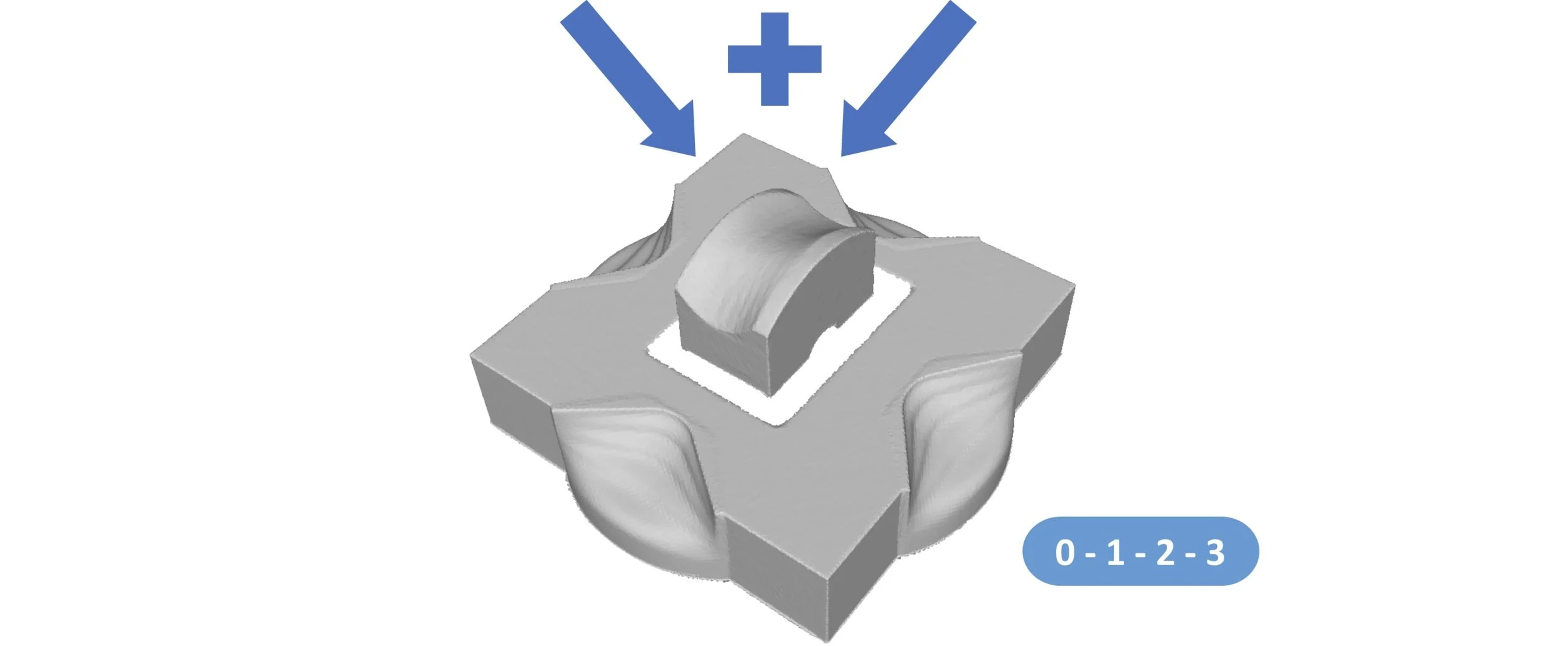
After removal of the initialization jig, a specimen piece is then securely clamped on to the platform. Note that the specimen has geometries that centre itself with respect to the rotary shaft of the robot.

Table Extension Frame
The frame clamps to a table using two lead screws, forming a cantilever structure extending from the table edge. This structure mimics the thigh of a patient, and the milling platform can be mounted to its distal end. The frame’s top plate height is adjustable to offer comfortable operation for robot operators of different statures. Threaded holes are also tapped at its distal bottom so that a camera tripod (with or without a tripod head) could be mounted for additional structural support.

Together, the milling platform and the extension frame can be configured into right-side or left-side medial UKA. The configuration can even be changed without re-initializing the robot.


Laser Scanning and Post Processing
Following the robot-guided milling experiments, the resultant specimen surfaces are digitized using laser scanning technique. The laser scanner was properly calibrated prior to scanning. Accuracy and precision of scanning and post-processing pipeline were both validated in separate studies performed earlier.

Laser Scanning Jig
Due to scanner’s field of view and line of sight limitations, multiple shots need to be stitched together to completely capture the geometry. Furthermore, the scanned surfaces need to be registered to a common coordinate system in order to be further analyzed and compared. However, cleaning individual scans and performing multiple stitching operations could severely lengthen post-processing time. I thus designed and fabricated a scanning jig to include special geometric features in scans to assist the software in performing shot-to-shot stitching. The jig successfully reduced the required shots to 4. The jig also contains reference geometries used for coordinate registration.

The specimen’s position is defined by its contacts with the jig’s reference edges, as shown by the red lines. There is also a spring-loaded holding mechanism that maintains these contacts throughout the scanning process.

At the jig bottom, locating pins and a step feature can be found. The pins match the scanner turntable groove and thus ensure consistent centring of the jig. The pins are magnetically attached and can be removed for use with other scanner models. The step feature creates a physical gap between the jig bottom and the turntable top, thereby eliminating scanning noise at the jig’s bottom edges.


Processing of Scanned Surfaces
I planned and performed the post-processing procedure which includes:
Delete undesired scanning noise from the edges of each individual shots.
Align and stitch together nearby shots by applying iterative closest point (ICP) algorithm at overlapping regions. The algorithm minimizes the the positional differences between the two mesh surfaces.
Clean over-lapping meshes at the region of interest, the milled area.

Coordinate Registration of Processed Surfaces
By running ICP algorithm on 3 planes on the scanning jig surface, a transformation is calculated and applied to the entire processed surface to register it to the desired common coordinate system. For this procedure, blue ideal reference planes (created with 3D CAD) are used as the ICP registration targets.

Comparison between the Processed Surfaces and the Ground-truth CAD Surface
To assess accuracy of the milling operation, I compared the scanned combined-curved and tri-planar surfaces to their respective ground-truth CAD surfaces. Furthermore, within each type of virtual-fixture, cross-comparisons are performed for different sets of scanned specimens to estimate the robot’s milling precision. The assessments are performed using cloud-mesh distance calculation. The algorithm calculates the closest (signed) distance from a point cloud surface to a reference mesh surface.

Scanned surfaces are trimmed to regions of interest and then sampled into point clouds.

The green region, where the original virtual-fixture surface model intersects the CAD specimen model, is extracted and converted to reference mesh surface.

Accuracy Result for One of the Milled Specimens
The result visualizes the deviation pattern on the milled surface, as shown in the left figure. Negative distance or blue denotes over-milling, while positive distance or red denotes under-milling. The deviation data is also imported to MATLAB to generate histogram (light blue), cumulative distribution function (orange), and other statistical values that are shown in the right figure. For this particular example, the mean deviation is -0.22 mm and the RMS deviation is 0.33 mm.